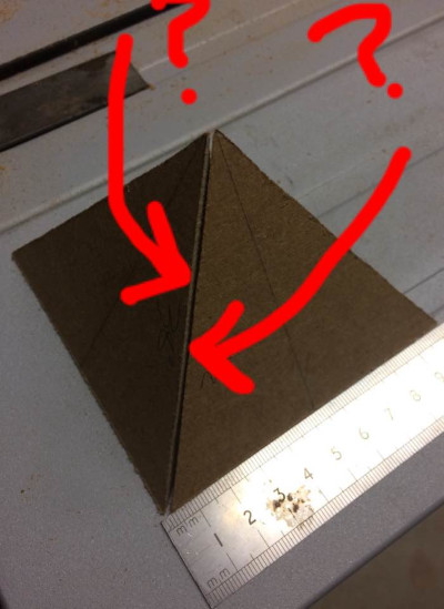
Reasoning about Pyramid Miter Joints

Someone pestered me with a question about how to calculate proper joint angles when building a square-based, equilateral pyramid. They wanted to know the angle to cut to form a miter joint between the adjacent triangular faces and also between the base and the bottom edge of each triangle.

This was a nice wee puzzle, and I think the graphing would make a nice excuse to test out numpy/matplotlib. Why not write it up then?

We can tackle this in two main steps:

We calculate how each triangular face is sloped inwards towards the apex (finding the join angle for the bottom edges) and then…
We think of two adjacent triangular faces as two intersecting planes (forget they are triangles at all!) to find the join angle between triangular faces.

As we go through how this works, I’ll include the python code I used to generate the figures (secret sauce: I exported this from a Jupyter notebook…). Just a little setup code for plotting before we dive in:

import math as m
import numpy as np
from numpy import *
from matplotlib import pyplot as plt
from mpl_toolkits.mplot3d import Axes3D
from matplotlib.patches import FancyArrowPatch
from mpl_toolkits.mplot3d import proj3d
from matplotlib import cm

class Arrow3D(FancyArrowPatch):
    def __init__(self, xs, ys, zs, *args, **kwargs):
        FancyArrowPatch.__init__(self, (0,0), (0,0), *args, **kwargs)
        self._verts3d = xs, ys, zs

    def draw(self, renderer):
        xs3d, ys3d, zs3d = self._verts3d
        xs, ys, zs = proj3d.proj_transform(xs3d, ys3d, zs3d, renderer.M)
        self.set_positions((xs[0],ys[0]),(xs[1],ys[1]))
        FancyArrowPatch.draw(self, renderer)
       
%matplotlib inline
a = 100

Calculating bottom join angle

Three sub steps here:

Consider one triangular face in the abstract. Calculate it’s height
Find the angle all triangular faces must be sloped at in order to fit around the base, touching tips at the apex
Find the height of this apex

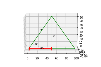
Start by looking at one triangular face in isolation to find it’s height. Remember it’s equilateral so we know the length of each edge, but not the height (yet).

fig = plt.figure()
ax = fig.add_subplot(111, projection='3d')

X1, Y1, Z1 = [0,a,a/2,0], [0,0,0,0], [0,0,a*m.sqrt(3)/2,0]
ax.plot_wireframe(X1, Y1, Z1, rstride=10, cstride=10, color='g')
ax.plot_wireframe([a/2,a/2], [0,0], [0,a*m.sqrt(3)/2], lineStyles='--', color='g')
ax.text(a/4, 0, 0, "a/2")
ax.text(a/4, 0, a/2, "a")
ax.text(a/2, 0, a/3, " b")
ax.text(a/10, 0, a/10, "60°")
ax.add_artist(Arrow3D([0,a/2], [0,0], [0,0], mutation_scale=5, lw=3, arrowstyle="|-|", color="r"))
ax.view_init(elev=10., azim=-90)
plt.show()

png

So, finding height, \(b\), in terms of length, \(a\):

\[\begin{aligned} sin(60°) &= \frac{b}{a}\\\\ \frac{\sqrt{3}}{2} &= \frac{b}{a}\\\\ b &= a \frac{\sqrt{3}}{2} \end{aligned}\]

Easy. So now we can look at how the 4 triangular faces are composed around the square base.

fig = plt.figure()
ax = fig.add_subplot(111, projection='3d')

apexz = a/m.sqrt(2)
ax.plot_wireframe([0,a,a/2,0],[a/2,a/2,a/2,a/2], [0,0,apexz,0], lw=8)
ax.plot_wireframe([0,0,a,a,0],[0,a,a,0,0],[0,0,0,0,0])
ax.plot_wireframe([0,0,a/2,0],[0,a,a/2,0], [0,0,apexz,0], color='g')
ax.plot_wireframe([a,a,a/2,a],[0,a,a/2,0], [0,0,apexz,0], color='g')
ax.text(a/4, a/2, 0, "a/2")
ax.text(a/10,a/2,a/20,"$\Theta_b$")
ax.text(a/2,a/2,apexz/2,"H")
ax.text(a/4,a/2,apexz/2,"b")
ax.add_artist(Arrow3D([0,a/2], [a/2,a/2], [0,0], mutation_scale=5, lw=3, arrowstyle="|-|", color="r"))
ax.add_artist(Arrow3D([a/2,a/2], [a/2,a/2], [0,apexz], mutation_scale=5, lw=3, arrowstyle="|-|", color="r"))
ax.view_init(elev=20., azim=-70)
plt.show()

png

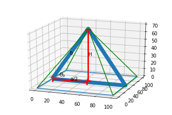
The thick blue line is down the middle of the base and bisects two opposing triangles. We know that the distance between the bottom of the opposing triangles must be \(a\) because it needs to fit another identical triangle to complete the pyramid! That’s how we get the distance to the mid-point as \(a/2\).

To find the bottom angle, \(\theta_b\), we use some more simple trig and our previous equation for \(b\).

\[\begin{aligned} cos\theta_b &= \frac{a/2}{b}\\\\ &= \frac{a/2}{a\sqrt{3}/2}\\\\ &= \frac{1}{\sqrt{3}}\\\\ \theta_b &= 54.74° \end{aligned}\]

Each triangle face sits at 54.74° from the horizontal, so we need to cut away 35.26° from the bottom edge. The maths was simple, but the answer seems already bit unintuitive. Think most folk would guess 45° or 60°…

Now we can also calculate the height of the apex of the pyramid using the Pythagorean theorem. This will help us a lot later on.

\[\begin{aligned} b^2 &= (\frac{a}{2})^2 + H^2\\\\ H^2 &= b^2 - (\frac{a}{2})^2\\\\ &= (\frac{a\sqrt{3}}{2})^2 - \frac{a^2}{4}\\\\ &= \frac{a^2}{2}\\\\ H &= \frac{a}{\sqrt{2}} \end{aligned}\]

Now we have the apex height, we have all the information we need to model two adjacent triangular faces as planes. Once we do this, we can calculate the join angle between triangular faces.

Calculating side join angles

We want to find the angle between two adjacent triangular faces as they meet. The easiest way I can think of for this is to describe each face as a plane and work out the angle of intersection between the planes. The fact these are triangles and not infinite planes doesn’t really matter.

fig = plt.figure()
ax = fig.add_subplot(111, projection='3d')

apexz = a/m.sqrt(2)
ax.plot_wireframe([0,0,a,a,0],[0,a,a,0,0],[0,0,0,0,0])
ax.plot_wireframe([0,a,a/2,0],[0,0,a/2,0], [0,0,apexz,0], color='g',lw=3)
ax.plot_wireframe([0,0,a/2,0],[0,a,a/2,0], [0,0,apexz,0], color='y',lw=3)
ax.plot_wireframe([a/2,a/2], [a/2,a/2], [0,a/m.sqrt(2)], lineStyles='--', color='b')
ax.add_artist(Arrow3D([-a/20,-a/20], [0,a], [0,0], mutation_scale=20, lw=3, arrowstyle="->", color="r"))
ax.text(-a/20,a/2,0,"$v_a$")
ax.add_artist(Arrow3D([0,a], [-a/20,-a/20], [0,0], mutation_scale=20, lw=3, arrowstyle="->", color="r"))
ax.text(a/2,-a/20,0,"$v_b$")
ax.add_artist(Arrow3D([0+a/20,a/2+a/20], [0,a/2], [0,apexz], mutation_scale=20, lw=3, arrowstyle="->", color="r"))
ax.text(a/4,a/4,apexz/2,"$v_c$")
ax.text(0,0,0,"(0,0,0)")
ax.text(a,0,0,"(a,0,0)")
ax.text(0,a,0,"(0,a,0)")
ax.text(a/2,a/2,a/sqrt(2),"(a/2,a/2,a/sqrt(2))$")
ax.view_init(elev=30., azim=-120)
plt.show()

png

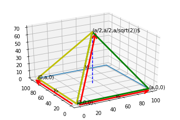
We can define the two planes given the three vectors shown above (\(v_1, v_2,\) and \(v_3\)). The plane 1 (yellow) is composed of \(v_a\) and \(v_c\) while plane 2 (green) is composed of \(v_b\) and \(v_c\).

We only actually need the normal of each plane and we can get it from these vectors!

\[\begin{aligned} n_1 &= v_a \times v_c\\\\ &= det\begin{bmatrix}i&j&k\\\\v_{ai}&v_{aj}&v_{ak}\\\\v_{ci}&v_{cj}&v_{ck}\end{bmatrix}\\\\ &= (v_{aj}v_{ck}-v_{ak}v_{cj})i-(v_{ai}v_{ck}-v_{ak}v_{ci})j+(v_{ai}v_{cj}-v_{aj}v_{ci})k\\\\ &= (0-0)i-(a\frac{a}{2}-0)k+(a\frac{a}{\sqrt{2}}-0)k\\\\ &= [0,-\frac{a^2}{2}, \frac{a^2}{\sqrt{2}}] \end{aligned}\]

And again for plane 2:

\[\begin{aligned} n_2 &= v_b \times v_c\\\\ &= [-\frac{a^2}{\sqrt{2}},\frac{a^2}{2}, 0] \end{aligned}\]

Now that we have both normals we can find the angle of intersection between the planes with as so:

\[\begin{aligned} cos\theta_c &= \frac{n_1\cdot n_2}{|n_1||n_2|}\\\\ &= \frac{0-\frac{a^2}{2}\frac{a^2}{2}+0}{\sqrt{0+(\frac{a^2}{2})^2+(\frac{a^2}{\sqrt{2}})^2}\sqrt{(\frac{a^2}{\sqrt{2}})^2+(\frac{a^2}{2})^2+0}}\\\\ &= \frac{-\frac{a^4}{4}}{\frac{3a^4}{4}}\\\\ &= -\frac{1}{3}\\\\ \theta_c &= 109.5° \end{aligned}\]

So the angle between the two planes (our two adjacent triangular faces) is 109.5°, requiring a cut a away of 35.25° on each side.

Job done! Yet to hear back if this worked in practice, but the join angles seem to be backup up here. Anyway, nice wee problem which proves less intuitive than I expected.

Cheers.